1 Edificaciones

Análisis de los datos Google-Microsoft-OSM

Mostrar código

import matplotlib.pyplot as plt

from shapely.geometry import box
import geopandas as gpd
import os


from matplotlib_map_utils import north_arrow, scale_bar


import contextily as cx


import pandas as pd
import contextily as ctx


import boto3
import duckdb
import s2sphere
from botocore.config import Config


from io import BytesIO
from owslib.wfs import WebFeatureService


USE_CRS = "EPSG:5349"  # POSGAR 2007 / Argentina 4
WEB_MERCATOR_CRS = "EPSG:3857"  # visualización
WGS84_CRS = "EPSG:4326"  # para llamadas API

BASE_RUTA = "/home/nissim/Documents/dev/fulbright/ciut-riesgo"
DATA_RUTA = f"{BASE_RUTA}/notebooks/data"
PARTIDOS_RUTA = f"{DATA_RUTA}/pba_partidos.geojson"
EDIFICACIONES_RUTA = f"{BASE_RUTA}/notebooks/edificaciones_filtered.parquet"

PARTIDOS_WFS_URL = "https://geo.arba.gov.ar/geoserver/idera/wfs"

Mostrar código

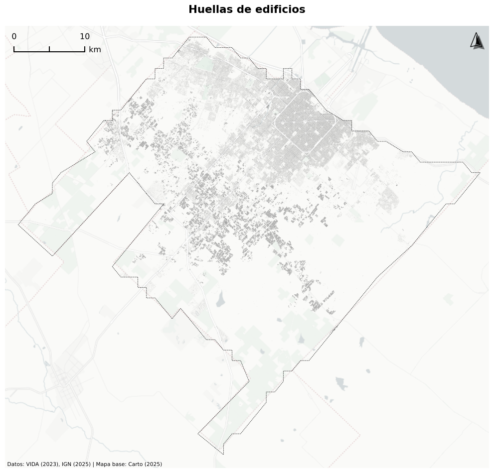
if os.path.exists(PARTIDOS_RUTA):
    print("Cargando datos de partidos existentes...")
    partidos = gpd.read_file(PARTIDOS_RUTA)
else:
    print("Descargando datos de partidos desde servicio WFS...")

    # Conectar al servicio WFS
    wfs = WebFeatureService(url=PARTIDOS_WFS_URL, version="2.0.0")

    # Descargar la capa de departamentos
    response = wfs.getfeature(typename="idera:Departamento", srsname="EPSG:5347")

    # Convertir a GeoDataFrame
    partidos = gpd.read_file(BytesIO(response.read()))

    # Guardar para uso futuro
    partidos.to_file(PARTIDOS_RUTA, driver="GeoJSON")
    print(f"Descargados {len(partidos)} partidos")

partidos = partidos.to_crs(USE_CRS)
aoi = partidos[partidos["fna"] == "Partido de La Plata"]

# Obtener la geometría principal
main_geom = aoi.geometry.iloc[0]

# Si es un MultiPolygon, mantener solo el polígono más grande (el partido principal)
# Esto elimina la pequeña isla que aparece en los datos
if main_geom.geom_type == "MultiPolygon":
    # Obtener todos los polígonos y mantener el que tenga mayor área
    largest_polygon = max(main_geom.geoms, key=lambda p: p.area)
    aoi = aoi.copy()  # Crear una copia para evitar SettingWithCopyWarning
    aoi.loc[aoi.index[0], "geometry"] = largest_polygon

aoi_bbox = aoi.geometry.iloc[0]

if os.path.exists(EDIFICACIONES_RUTA):
    print("Cargando datos de edificaciones existentes...")
    edificaciones = gpd.read_parquet(EDIFICACIONES_RUTA)
else:
    print("Obteniendo datos de edificaciones del dataset VIDA...")

    # Paso 1: Obtener el punto central de La Plata en coordenadas WGS84
    aoi_buffered = aoi.buffer(500)  # Agregar buffer de 500m para obtener datos
    center = aoi_buffered.to_crs(WEB_MERCATOR_CRS).union_all().centroid
    center_wgs84 = (
        gpd.GeoDataFrame(geometry=[center], crs=WEB_MERCATOR_CRS)
        .to_crs(WGS84_CRS)
        .geometry.iloc[0]
    )
    print(f"Coordenadas del centro: {center_wgs84.y:.4f}, {center_wgs84.x:.4f}")

    # Paso 2: Encontrar la celda S2 apropiada para particionamiento espacial
    cell = s2sphere.CellId.from_lat_lng(
        s2sphere.LatLng.from_degrees(center_wgs84.y, center_wgs84.x)
    ).parent(10)
    print(f"ID de celda S2: {cell.id()}")

    # Paso 3: Obtener bounding box en WGS84 para filtrado espacial
    bounds = aoi_buffered.to_crs(WGS84_CRS).total_bounds
    print(f"Caja delimitadora: {bounds}")

    # Paso 4: Conectar a S3 y encontrar particiones disponibles
    s3 = boto3.client(
        "s3",
        endpoint_url="https://data.source.coop",
        aws_access_key_id="",
        aws_secret_access_key="",
        config=Config(s3={"addressing_style": "path"}),
    )

    # Obtener lista de particiones S2 disponibles
    partitions = {
        obj["Key"].split("/")[-1].replace(".parquet", "")
        for obj in s3.list_objects_v2(
            Bucket="vida",
            Prefix="google-microsoft-osm-open-buildings/geoparquet/by_country_s2/country_iso=ARG/",
        ).get("Contents", [])
    }
    print(f"Encontradas {len(partitions)} particiones disponibles")

    # Paso 5: Encontrar la partición padre apropiada
    parent_id = next(
        str(cell.parent(level).id())
        for level in range(10, 0, -1)
        if str(cell.parent(level).id()) in partitions
    )
    print(f"Usando partición: {parent_id}")

    # Paso 6: Configurar DuckDB para consultas espaciales
    con = duckdb.connect()
    print("Configurando DuckDB con extensiones espaciales...")
    for cmd in [
        "INSTALL spatial",
        "LOAD spatial",
        "INSTALL httpfs",
        "LOAD httpfs",
        "SET s3_region='us-east-1'",
        "SET s3_endpoint='data.source.coop'",
        "SET s3_use_ssl=true",
        "SET s3_url_style='path'",
    ]:
        con.execute(cmd)

    # Paso 7: Consultar y filtrar edificaciones dentro de nuestra área de interés
    print("Consultando edificaciones dentro del área de La Plata...")
    query = f"""
    COPY (SELECT * FROM 's3://vida/google-microsoft-osm-open-buildings/geoparquet/by_country_s2/country_iso=ARG/{parent_id}.parquet'
          WHERE bbox.xmax >= {bounds[0]} AND bbox.xmin <= {bounds[2]} AND
                bbox.ymax >= {bounds[1]} AND bbox.ymin <= {bounds[3]}
    ) TO '{EDIFICACIONES_RUTA}' (FORMAT PARQUET);
    """

    con.execute(query)

    # Paso 8: Cargar los datos filtrados y convertir a GeoDataFrame
    df = pd.read_parquet(EDIFICACIONES_RUTA)
    df["geometry"] = gpd.GeoSeries.from_wkb(df["geometry"])
    edificaciones = gpd.GeoDataFrame(df, geometry="geometry", crs=WGS84_CRS)

    print(f"Obtenidas {len(edificaciones)} edificaciones")
    con.close()


# Filtrar edificaciones para incluir solo las que están dentro de los límites de La Plata
edificaciones_proj = edificaciones.to_crs(USE_CRS)
edificaciones_proj = edificaciones_proj[
    edificaciones_proj.geometry.intersects(aoi_bbox)
]

Cargando datos de partidos existentes...
Cargando datos de edificaciones existentes...

Mostrar código

# Obtener límites de La Plata y convertir a Web Mercator para visualización
aoi_bounds = aoi_bbox.bounds
temp_bounds = gpd.GeoDataFrame(
    geometry=[box(aoi_bounds[0], aoi_bounds[1], aoi_bounds[2], aoi_bounds[3])],
    crs=USE_CRS,
)
bounds_3857 = temp_bounds.to_crs(WEB_MERCATOR_CRS).total_bounds

fig, ax = plt.subplots(figsize=(12, 10))
ax.set_xlim(bounds_3857[0] - 500, bounds_3857[2] + 500)
ax.set_ylim(bounds_3857[1] - 500, bounds_3857[3] + 500)

cx.add_basemap(
    ax,
    crs=WEB_MERCATOR_CRS,
    source=ctx.providers.CartoDB.PositronNoLabels,
    attribution="Datos: VIDA (2023), IGN (2025) | Mapa base: Carto (2025)",
)

scale_bar(
    ax=ax,
    location="upper left",
    style="ticks",
    bar={
        "projection": "EPSG:3857",
        "tickcolors": "black",
        "basecolors": "black",
        "minor_type": "none",
        "length": 0.20,
    },
    labels={"style": "first_last"},
)

# Add north arrow
north_arrow(
    ax,
    location="upper right",
    scale=0.3,
    rotation={"degrees": 0},
    base={"facecolor": "none", "edgecolor": "black", "linewidth": 1},
    fancy=True,
    shadow=True,
    label=False,
)

aoi_3857 = aoi.to_crs(WEB_MERCATOR_CRS)
aoi_3857.plot(
    ax=ax,
    facecolor="none",
    edgecolor="black",
    linewidth=0.5,
    linestyle="--",
    legend=False,
    zorder=5,
)

edificaciones_3857 = edificaciones_proj.to_crs(WEB_MERCATOR_CRS)
edificaciones_3857.plot(ax=ax, facecolor="grey", edgecolor="none", alpha=0.7)

ax.set_title("Huellas de edificios", fontsize=16, fontweight="bold", pad=20)
ax.set_axis_off()

plt.tight_layout()
plt.show()

Figure 1.1: Huellas de edificios en La Plata, PBA