2  Open Data for Cities and Climate

2.1 Objectives

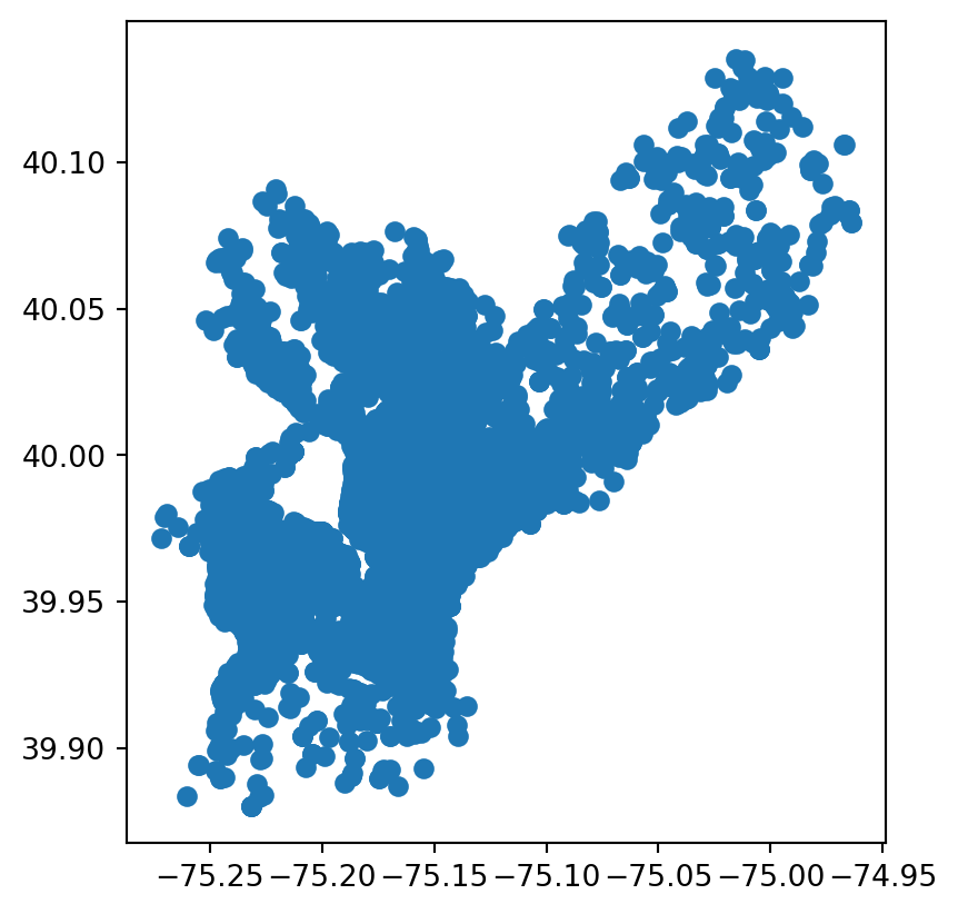
After completing this chapter, you will have an understanding of what open data is, common formats and platforms for accessing open geospatial data, and how to evaluate the quality and suitability of open datasets for local use.

2.2 What is Open Data?

This is a book about using data to help cities make better decisions about climate risk. While there are various potential sources for those data, in this book we focus on open data. Toward the end of this chapter, we’ll talk a bit about the complexities of what open data look like in the real world, but for now we’ll start with a basic working definition that open data is data that anyone can “freely access, use, modify, and share for any purpose” (Open Knowledge Foundation 2015). To clarify what this means, it might help to begin with a couple of concrete examples.

Here are some open data portals from the U.S. government, the government of India, and the government of the City of Buenos Aires:

Portal	Description
data.gov	U.S. federal open data portal
data.gov.in	India national open data portal
Catálogo de Datos GBA	Buenos Aires Province data catalog

If you click on one of the links and explore it, you’ll see many different datasets covering different time periods, regions, and topics. You’ll also likely notice that these three portals are all government portals, which isn’t an accident. The idea of publicly-accessible data is old, but the “open data” movement tends to refer to a particular initiative that emerged in the 2010s and focused primarily on open government data. As such, national, regional, and local governments are some of the main publishers of open data.

TipTry it yourself

Find an open data portal for your national, regional, or local government. What datasets does it offer? Can you find any data that might be useful for your work?

Beyond governments, open data are often published by quasi-governmental institutions like the United Nations, as well as by government-funded research organizations like the European Research Commission’s Joint Research Centre. Open data are also shared by many scientific researchers, not just for reproducibility but for real-world use. Here are some examples that are particularly relevant to urban climate risk:¹

Source	Description
OpenStreetMap	Community-generated geographic data; strong for roads and buildings in urban areas, but coverage and quality vary by region
Overture Maps	Open map data combining contributions from multiple sources into a single, validated dataset
Google Earth Engine	Platform for satellite imagery and geospatial analysis; free for research and non-commercial use
GEE Community Catalog	Community-curated datasets not in the official Earth Engine catalog; excellent for specialized climate data
OpenLandMap	Global environmental layers (soil, climate, vegetation) based on machine learning models
Source Cooperative	Community-driven data catalog emphasizing cloud-native formats and open science
Microsoft Planetary Computer	Curated earth observation data optimized for cloud-native analysis at scale
TUM Global Building Heights	Global building height dataset derived from remote sensing; useful for urban morphology and exposure modeling

As you can see, there’s a lot of open data out there–and, in fact, the quantities of available open data have been growing rapidly since the 2010s, and in particular now in the age of cloud storage and artificial intelligence. This raises the question: with all of that data out there, how do find what I need?

2.3 Where is Open Data?

What we’ve seen so far are examples of data portals, where are one of several kinds of spatial data infrastructure (SDI). An SDI is basically any place where open geospatial data can be found on the internet, such as catalogs, servers, web apps, or even just a list of pages. In this chapter, we’ll look at a few of the most common types of SDIs, including data portals, APIs, and cloud storage.

2.3.1 Data Portals

A data portal is a website that provides access to datasets, often with search and filtering capabilities. The purpose of a data portal is to make it easier for users to discover and access datasets relevant to their needs, so they usually provide metadata, such as descriptions, formats, and licensing information, and tools for previewing and downloading the data. Open data portals are a great place to start your search for data, as they’re designed primarily for easily searching through a catalog (or catalogs) of available data to find and acccess what you need.

Tip

Often, data portals don’t actually host the data itself. Instead, they provide a user interface to organize and navigate data, while storage is handled elsewhere, whether in databases, cloud storage, or other infrastructure.

Metadata is data that defines and describes other data. Usually it will include information like the title, publisher, publication, and description date for a dataset. It might also include schema information (i.e., what’s in the data itself), update frequency, licensing, contact information for the publisher, etc. Geospatial datasets usually have a unique set of metadata such as their bounding box and CRS.

Let’s take a look at an example. Here’s a dataset of building demolitions listed on the City of Philadelphia’s open data portal:

Building Demolitions, OpenDataPhilly

As expected, we can see a title, a description, and some metadata (created date, categories, a license, a maintainer and contact info). OpenDataPhilly also lists several options for how to access the data, including a visualization page (the HTML link), an API (more on this in a moment), and three flat file formats (CSV, shapefile, and GeoJSON).

2.3.2 Flat Files

A flat file is a file that you download once in its entirety. They can be used offline with no internet connection, and they don’t change unless the user manually edits them. The major benefit of flat files is their simplicity. What you see is what you get, and they are straightforward to access: you download them, search for them on your computer, and open them with your desktop GIS software or with a programming language.

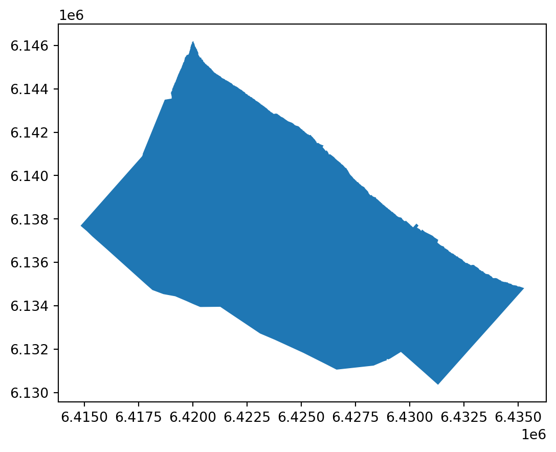
Here’s a quick example of accessing the buildings demolitions data as a flat file. We’ve downloaded the data as a GeoJSON and can simply open the file directly in Python (for a recap of this, see chapter 1).

import geopandas as gpd

building_demos = gpd.read_file("building_demolitions.geojson")
building_demos.plot()

Tip

Raster data also come in flat files, such as GeoTIFFs, netCDF, and ECW. Just like vector data, these can be downloaded and opened in Python, as covered in chapter 1.

While both vector and raster data can come in several flat file formats–each of which has its own strengths and limitations–tools like geopandas and rasterio make it easy to open all of these formats with a consistent interface.

As we mentioned, flat files have the virtue of simplicity, and for many geospatial practitioners, they will never need to go beyond downloading and analyzing flat files. But what if we want to work with a dataset that updates regularly? What if we want only part of a very large dataset, or we want to access the data progammatically, such as in a script? These are cases where flat files can come up short, and where we might turn instead to APIs.

2.3.3 APIs

In the simplest terms, an API is a structured way to ask a computer for something and get a response back.

What is an API? Source: roboleary.net

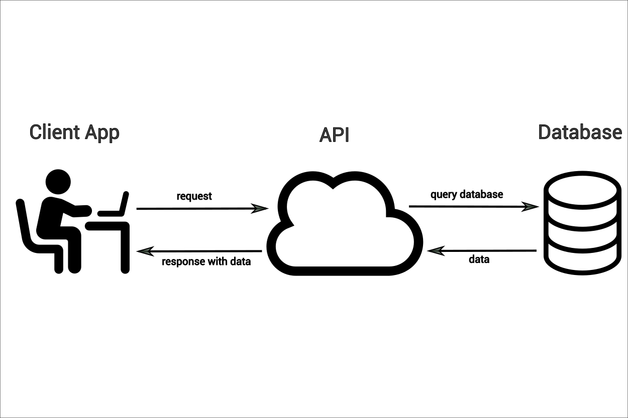
Let’s return to the example of our building demolitions data and dig a little deeper. When we right-click on the “GeoJSON” link, we get the following URL:

https://phl.carto.com/api/v2/sql?q=SELECT+*+FROM+demolitions&filename=demolitions&format=geojson&skipfields=cartodb_id.

This reveals something interesting: our “download” link is actually a query passed via API to a database. We can break it down in more detail:

• We are querying a SQL-style Carto database belonging to the City of Philadelphia (https://phl.carto.com/api/v2/sql)
• We are requesting data specifically from the demolitions table
• We are requesting that the response be returned as GeoJSON data (geojson)

In fact, if we right-click on the shapefile or CSV download links, we’ll see that the queries are almost identical, the only difference being that the shapefile query specifies shp instead of geojson, and the CSV query specifies csv and also needs to indicate the formatting of the geometry data (ST_Y(the_geom)+AS+lat,+ST_X(the_geom)+AS+lng). In other words, there aren’t actually three different files, but a single database that we access via API. This gives us another option for data access. Instead of downloading these data as a flat file, we can query them in Python to get the same results:

import requests
import geopandas as gpd

url = "https://phl.carto.com/api/v2/sql"
params = {
    "q": "SELECT * FROM demolitions",
    "format": "geojson",
    "skipfields": "cartodb_id",
}

response = requests.get(url, params=params)
gdf = gpd.GeoDataFrame.from_features(response.json())
gdf.plot()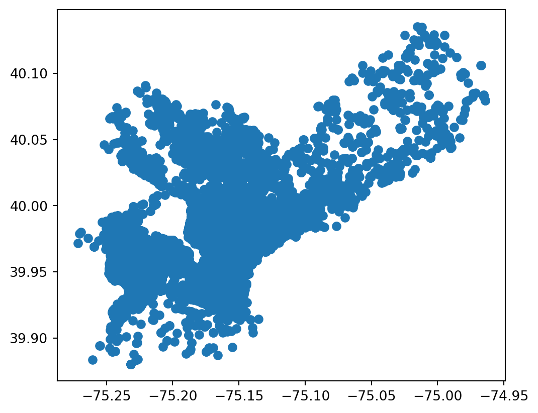

While a flat file is static, our query is not; each time we run it, the results will change depending on what’s in the database. And while static flat files are good for one-off analysis, APIs give us the opportunity to access data flexibly and programmatically, such as scripting regular data updates or filtering only for the data we need. In the example we’ve just seen, we’re connecting to a PostGIS database which can be queried via SQL. This is one flavor of API, but it’s specific to Carto, the vendor that provides it. In the open data world, you may run into many different kinds of APIs, each with their own quirks. We can’t be comprehensive, but let’s take a look at two more very common ones that are worth being familiar with.

2.3.3.1 WFS/WMS

Web Feature Services (WFS) and Web Map Services (WMS) are standardized APIs for sharing vector and raster features (respectively). These standards are maintained by the Open Geospatial Consortium (OGC) and are meant to facilitate consistent access and distribution patterns for open geospatial data. Since the standards and tooling are open source, they are the go-to for sharing geospatial data in much of the world, especially the Global South.

Let’s take a look at a simple example of accessing data via WFS. We’ll return to the partidos data from the Province of Buenos Aires that we looked at in chapter 1. This time, instead of loading the data from a pre-downloaded local copy, we’ll query it directly from the ARBA WFS server. Note that we can now pass our query directly to the server, limiting the response to just the Partido de Berisso ("CQL_FILTER": "fna='Partido de Berisso").

import requests
import geopandas as gpd

# We use requests instead of owslib here because owslib's WebFeatureService
# client doesn't support disabling SSL verification
url = "https://geo.arba.gov.ar/geoserver/idera/wfs"
params = {
    "service": "WFS",
    "version": "2.0.0",
    "request": "GetFeature",
    "typename": "idera:Departamento",
    "CQL_FILTER": "fna='Partido de Berisso'",
    "srsname": "EPSG:5347",
    "outputFormat": "application/json",
}

# verify=False because ARBA's SSL certificate is currently expired
response = requests.get(url, params=params, verify=False)
berisso = (
    gpd.GeoDataFrame.from_features(response.json())
    .set_crs("EPSG:5347")
    .to_crs("EPSG:5348")
)
berisso.plot()

/home/runner/work/datos-escala-humana/datos-escala-humana/.venv/lib/python3.12/site-packages/urllib3/connectionpool.py:1097: InsecureRequestWarning:

Unverified HTTPS request is being made to host 'geo.arba.gov.ar'. Adding certificate verification is strongly advised. See: https://urllib3.readthedocs.io/en/latest/advanced-usage.html#tls-warnings

For simplicity and clarity, we’re making this query via the requests library, as we did in the Carto example before and as we will in the Esri example in the next section. However, OGC also maintains owslib, a Python library for working with WFS/WMS. For details on how to use it, such as querying a WMS layer, see the official documentation.

2.3.3.2 Esri REST APIs

If you spend enough time working with geospatial data, you will inevitably come across Esri. While Esri’s products are proprietary (and therefore not open source), they are so widely used in the geospatial world that it’s basically impossible not to encounter them at some point. Much of the world’s geospatial data is stored in Esri servers, so it’s important to know how to access data via Esri’s own API. Here’s an example that is very similar to the WFS query above. As before, we’ll construct a query URL with parameters, make a request, and convert the results to a GeoDataFrame.

import requests
import geopandas as gpd
from shapely.geometry import shape

url = "https://services.arcgis.com/fLeGjb7u4uXqeF9q/arcgis/rest/services/Council_Districts_2024/FeatureServer/0/query"
params = {
    "where": "1=1",
    "outFields": "*",
    "f": "geojson",
}

response = requests.get(url, params=params)
gdf = gpd.GeoDataFrame.from_features(response.json())
gdf.plot()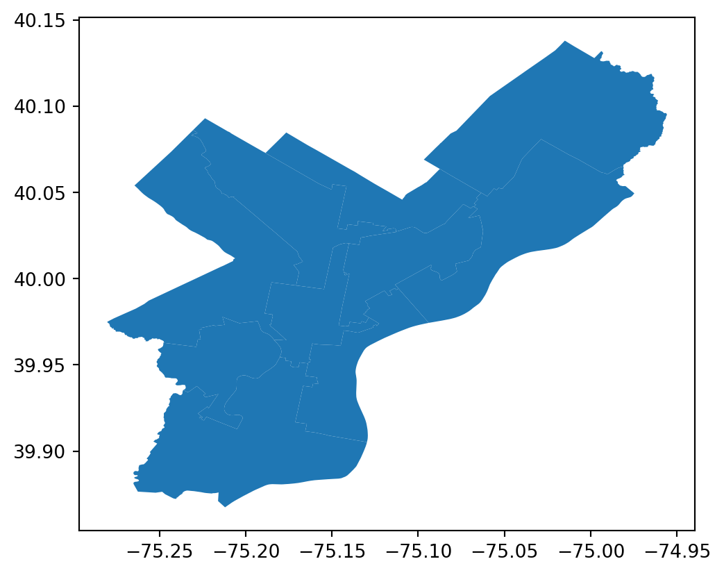

For more details on Esri REST API query syntax, see the official documentation. There are also several Python libraries that streamline extraction, such as esri2gpd and esri-dump, though neither is actively maintained. One of the authors of this book maintains geoparquet-io, a CLI tool and Python library that, among other features, makes it easy to extract data from ArcGIS feature services and convert the data to optimized geoparquet files (see the geoparquet.io extraction guide). It’s also often possible to simply download the data as a GeoJSON or Shapefile, as long as a download link is provided.

2.3.4 Cloud Storage

So far, we’ve discussed flat files and APIs as two different ways to access open data. These approaches work well for small- or medium-scale datasets, perhaps up to hundreds of gigabytes. But modern geospatial workflows—including many of the ones we’ll discuss in this book—often involve thousands or even millions of gigabytes of data. For workflows at this scale, traditional flat files and APIs simply aren’t appropriate; at best, they’re slow and cumbersome, and at worst, they make certain tasks literally impossible. This is where cloud storage and cloud-native file formats come in.

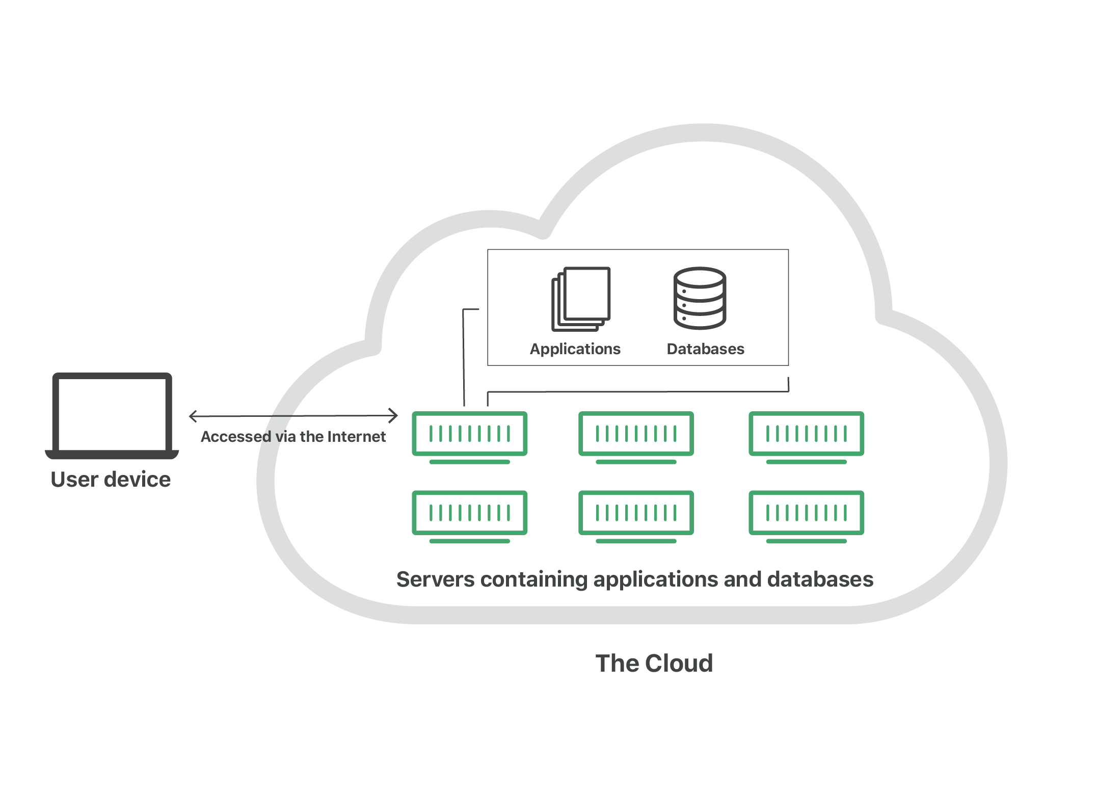
First, a definition: the cloud is nothing more than someone else’s computer, servers that your machine connects to over the internet. Accessing cloud infrastructure has an initial learning curve, and it requires a consistent internet connection, but it offers power, flexibility, scalability, and resilience that local storage cannot match.

What is the cloud? (Cloudflare 2025)

Here’s a concrete example to illustrate the how cloud storage improves on legacy approaches. Let’s say Carolina works as a GIS analyst for her local municipality, and she’s been asked to store 3.2 GB of cadastral data. Without cloud storage, she might need to purchase an external hard drive, which could cost $100 or more. The hard drive might hold 5 TB of data (or 5,000 GB), but if Carolina only ever uses 500 GB of that, she’s paying for 4,500 GB she’ll never use. On top of that, her options for sharing files are limited: she can either attach them to an email, if they’re small enough, or copy them to a USB stick and pass it along by hand. And, perhaps worst of all, if she loses the hard drive or something happens to it, everything on it is gone—there’s no backup, no distribution.

Contrast this with cloud storage. On platforms like Google Cloud or Amazon Web Services, storage costs around $0.025 per GB per month. At that price, Carolina’s 3.2 GB of cadastral data would cost her just under a dollar ($0.96, to be exact) per year. If she wants to share her data with a colleague, she can simply send them a URL to download or query the data directly. And there’s no risk of losing a hard drive, because she can access her data from anywhere she can sign into her cloud account.

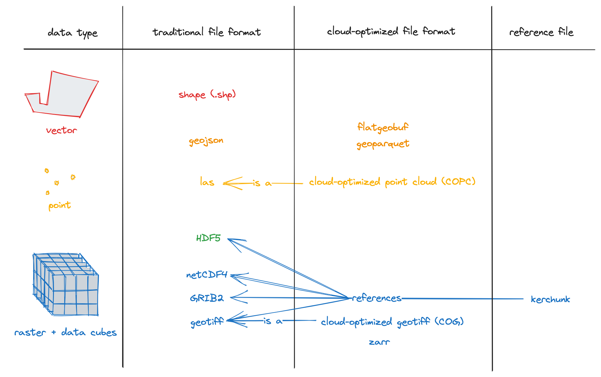
The cloud isn’t just about where you store your data; the how is also important. In recent years, several new file formats have emerged to make the most of the advantages of cloud storage. These are called cloud-optimized (or cloud-native) file formats, and they include cloud-optimized GeoTIFFs and Zarr for rasters, as well as GeoParquet, FlatGeobuf, and PMTiles for vectors. (To read more about these, see the Cloud-Optimized Geospatial Formats Guide.)

Cloud-Optimized File Formats

Cloud-native file types combine the simplicity of flat files with the flexility and scability of APIs, but to an even greater extent. They allow users to store millions of gigabytes of data while accessing just the portions they need. In other words, instead of having to download the entire file, you download just the data that matters to you. Here’s an example.

In the last chapter, we loaded Mapbiomas land cover data. The original data are stored as a cloud-optimized GeoTIFF in a Google Cloud bucket. (In other words, a cloud-native file in cloud storage.) The full raster is ~430 MB, or a bit under half a gigabyte. We can get a near-intantaneous map of the data for all of Argentina using overviews:

import rioxarray as rio
import numpy as np
from matplotlib.colors import ListedColormap, BoundaryNorm

categories = {
    "Closed woody": {"ids": [3], "color": "#1f8d49"},
    "Open woody": {"ids": [4], "color": "#7dc975"},
    "Sparse woody": {"ids": [45], "color": "#807a40"},
    "Flooded woody": {"ids": [6], "color": "#026975"},
    "Flooded non-woody vegetation": {"ids": [11], "color": "#519799"},
    "Grassland": {"ids": [12], "color": "#d6bc74"},
    "Steppe": {"ids": [63], "color": "#ebf8b5"},
    "Pasture": {"ids": [15], "color": "#edde8e"},
    "Agriculture": {"ids": [18], "color": "#e974ed"},
    "Forest plantation": {"ids": [9], "color": "#7a5900"},
    "Shrub crop": {"ids": [36], "color": "#d082de"},
    "Agricultural mosaic": {"ids": [21], "color": "#ffefc3"},
    "Non-vegetated area": {"ids": [22], "color": "#d4271e"},
    "River, lake or ocean": {"ids": [33], "color": "#2532e4"},
    "Ice and surface snow": {"ids": [34], "color": "#93dfe6"},
    "Not observed": {"ids": [27], "color": "#ffffff"},
}

colors_by_id = {
    id_: info["color"] for info in categories.values() for id_ in info["ids"]
}
sorted_ids = sorted(colors_by_id.keys())
lc_cmap = ListedColormap([colors_by_id[i] for i in sorted_ids])
lc_norm = BoundaryNorm(sorted_ids + [max(sorted_ids) + 1], lc_cmap.N)

suelo_2022_ruta = "https://storage.googleapis.com/mapbiomas-public/initiatives/argentina/collection-1/coverage/argentina_coverage_2022.tif"
overview = rio.open_rasterio(suelo_2022_ruta, overview_level=4).squeeze()
overview = overview.where((overview != 0) & (~np.isnan(overview)))

overview.plot(cmap=lc_cmap, norm=lc_norm, add_colorbar=False)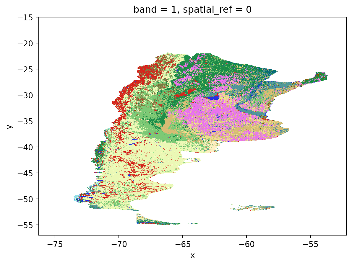

The real magic comes when we load just the section we need, in this case, corresponding to the Partido of Berisso, which we mapped in the previous section on WFS. Thanks to the magic of cloud-native workflows, we are only pulling 1.69 MB of data–just 0.4% of the full file size!

import rioxarray as rio
import numpy as np

# Reproject Berisso to raster CRS (WGS84)
berisso_wgs84 = berisso.to_crs("EPSG:4326")

# Clip raster to Berisso (full resolution, not overview)
berisso_lc = (
    rio.open_rasterio(suelo_2022_ruta)
    .rio.clip(berisso_wgs84.geometry, from_disk=True)
    .squeeze()
)

# Mask nodata
berisso_lc = berisso_lc.where((berisso_lc != 0) & (~np.isnan(berisso_lc)))

# Size in MB (actual bytes transferred ≈ uncompressed clip size)
size_mb = berisso_lc.nbytes / (1024**2)
print(f"Berisso clip: {size_mb:.2f} MB")

# Plot
berisso_lc.plot(cmap=lc_cmap, norm=lc_norm, add_colorbar=False)

Berisso clip: 1.69 MB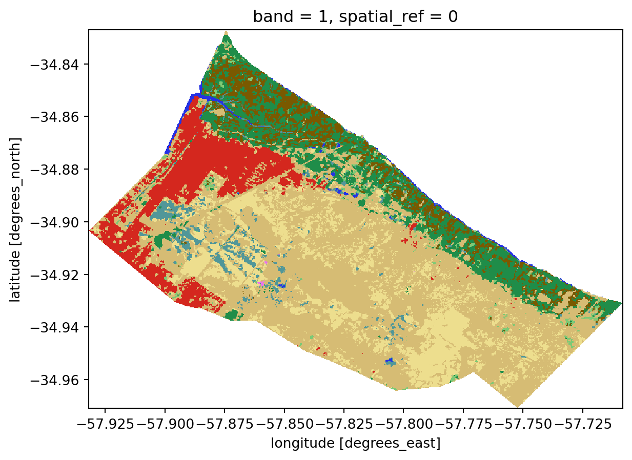

For climate risk analyses with global datasets, the ability to pull only the data you need is essential; if we had to download the entirety of CMIP6 data just to run an analysis for a small city in Bolivia, it would be literally impossible. Thanks to cloud-native geospatial tooling, however, it is now easy to access gold-standard climate data even on a normal office laptop.

2.4 Data Quality and Fitness for Use

As the examples above suggest, there is a lot of open data in the world, and no two datasets are quite alike. The definition we cited at the beginning of this chapter makes the idea sound simple in theory, but in practice it gets complicated quickly. That’s why it’s especially important to be able to carefully evaluate the quality and trustworthiness of an open dataset before building anything on top of it. Here are several questions to ask yourself.

First, is the dataset maintained? It is common to find “orphaned” datasets online–data that were published years ago and are no longer actively maintained by anyone. This lack of maintainence isn’t necessarily a problem if the data is in a final state, but it means that no one is accountable to answer questions you may have about the data. Often, it simply means that the data were superseded and you should look for a newer version of the dataset.

Second, how complete is the data documentation? Good documentation tells you who published the data and when, provides contact information for the publisher and/or maintainer, and includes key information such as metadata, known limitations, and guidance on interpretation. Without good documentation, it is very hard to know if you’re using a dataset as intended, which can lead to all kinds of problems when trying to make sound decisions based on the data.

Important

A key part of dataset documentation is the license. Common open licenses like Creative Commons (CC-BY, CC-BY-SA) and the Open Database License (ODbL) are generally permissive, but not all licenses are equal, and many have specific requirements about how you use, attribute, and share the data.

Related to documentation is the question of data quality. Well-documented datasets include quantitative and/or qualitative assessments of how accurate and reliable the data are. Validation and uncertainty metrics should tell you what the strengths and limitations of the dataset are, and give you a sense of what you can and can’t be confident in when using it.

Global Land Cover Datasets Compared. Source: Land Carbon Lab

Important

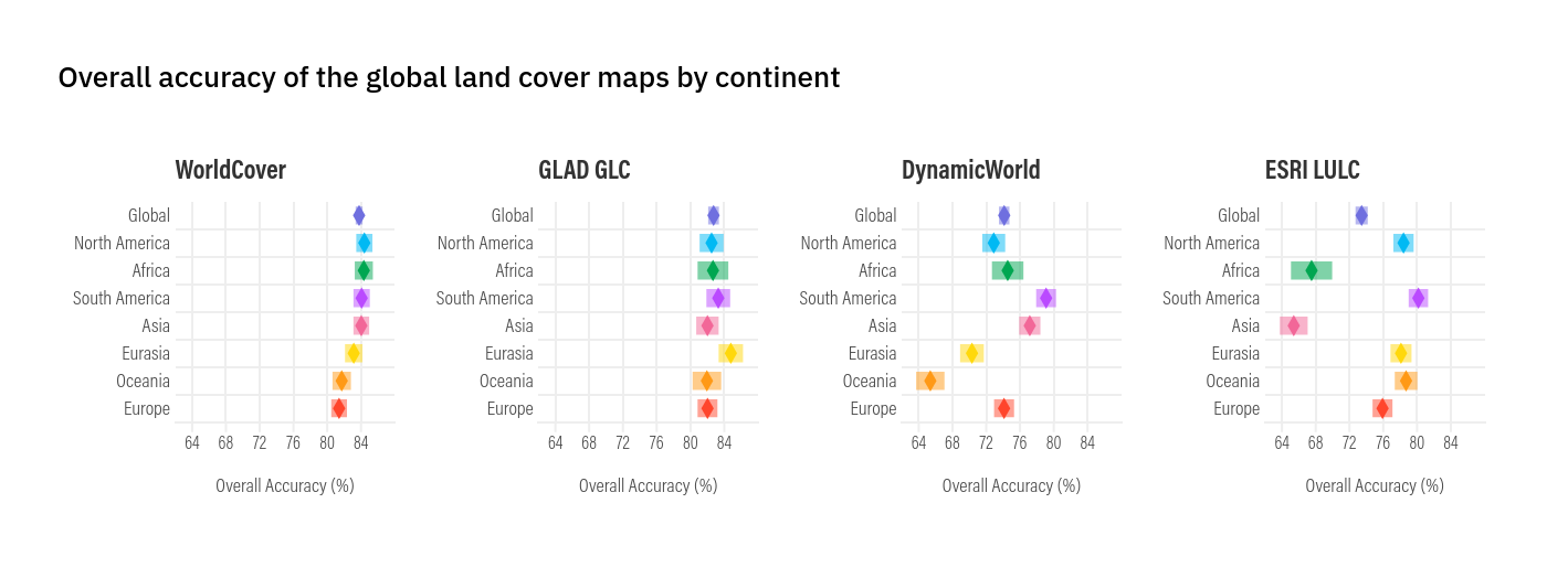
When reading a global dataset’s validation report, be mindful to how it performs in your specific region. Due to variation and/or bias in their training data, global datasets usually perform better in some countries or regions than others. Keep this in mind when selecting the most appropriate data sources for your use case.

In addition to checking documentation, it’s the responsibility of the data user to do their own validation, especially when they understand the local context. If you’re trying to decide which global land cover map is best suited for use in your city, you should open it in software like QGIS and actually compare it to high-resolution basemaps and your own understanding of what your city is like. If you’re using a global flood hazard model, compare it to a map of local flood defenses, which are often hard to factor into global flooding models. If you’re comparing two datasets, try to understand where and why they differ. In short, do not use data blindly.

Lastly, ask yourself if the data are the right tool for the job you’re trying to do. In other words, are they fit for use? Even “accurate” data, when applied to questions they weren’t meant to answer, can lead to bad outcomes. Using riverine flood hazard data in a place that only has pluvial flash flooding would give you totally misleading estimates of flood risk. VIIRS/FIRMS fire observations are helpful for mapping wildfires at a large scale, but aren’t always sensitive enough to pick up small roadside wildfires when they’ve just started. Ideally, datasets would include explicit guidance on what they should and shouldn’t be used for, but in practice this is rare. The best approach is to proceed with caution, look for prior precedent of how the dataset has been applied, and consult subject matter experts whenever you have doubts. Good geospatial work, in the end, depends as much on knowing the limits of your data as on knowing how to process it.

2.5 Why Use Open Data? A Case Study

It’s a truism that local data are better than global data. This is often true: locally-collected datasets are generally based on a more complete understanding of the local context than global datasets can be. However, this is changing rapidly, driven especially by massive improvements in artificial intelligence that are enabling more and more accurate open, global datasets. Furthermore, the quality of local datasets is often hampered by limited resources; especially in Global South countries, demographers, statisticians, and other producers are often hampered by under-funding, political instability, and numerous other challenges that impact the quality and availability of local data. As a result, open global datasets increasingly provide valuable supplements to or even replacements for local data, and can reveal crucial information. Here’s an illustrative case study.

The greater La Plata region in Argentina has a number of informal settlements exposed to flood hazards. In previous studies (Romanazzi et al. 2019), the city and the Universidad Nacional de La Plata had estimated the population of these informal settlements based on REBANAP data, Argentina’s official census of informal settlements. Although RENABAP provides the authoritative estimates of informal settlement populations, they are not fine-grained (they simply estimate the number of families per settlement, with no estimate of population distribution within settlements), and have another of methdological limitations. The most recent data, for example, published in 2023, include estimates based on surveys completed as far back as 2016. In the context of informal settlements–where population changes are swift and sometimes unpredcitable–this can lead to completely inaccurate population counts and therefore prevent local governments from adequately providing services.

As part of broader research work in Argentina, we worked in 2025 to pull open building footprints to compare to RENABAP data in La Plata. Our findings were stark: the RENABAP data may underestimate the real population in these settlements by roughly 40%. In one extreme case, we found an informal settlement that RENABAP estimated was inhabited by 330 families–but satellite imagery showed that it contained more than four thousand building footprints.

Example of Informal Settlement, La Plata, Argentina

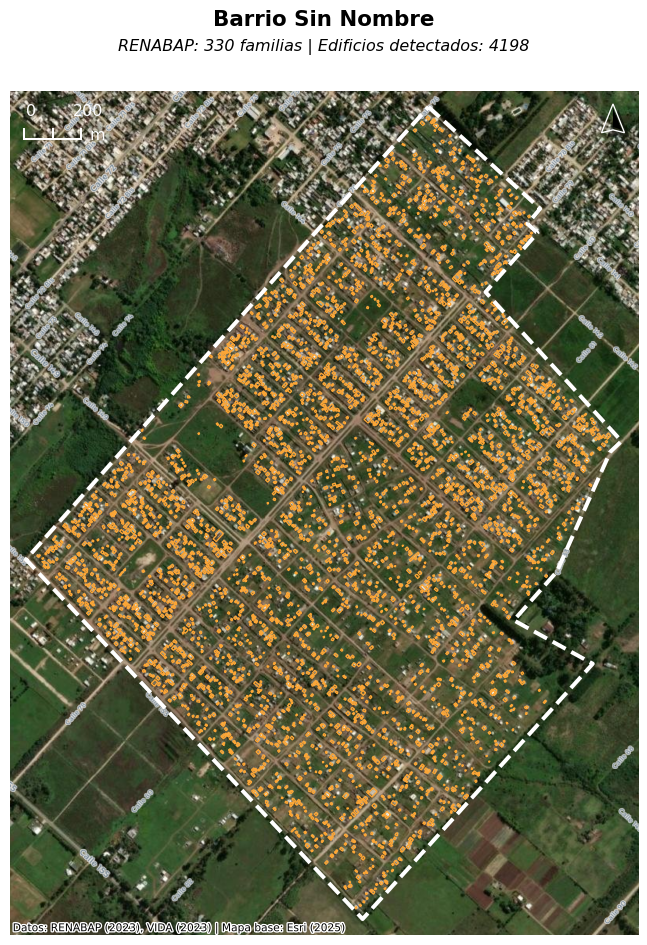
We ultimately estimated that as many as 100,000 people may be missing from population surveys of La Plata’s informal settlements, key information which has now been incorporated into La Plata’s first-ever municipal plan, and will be used to inform future decisions such as flood risk planning.

The lesson here is not that RENABAP is a failure and local data are irrelevant; rather, this is a clear example of how open global datasets can be used to supplement local datasets to refine and improve them, especially in contexts where limited resources or governance challenges may render official datasets unreliable.

2.6 Conclusion

In this chapter, we’ve covered what open data is, where and how to access it, and how to think critically about data quality and fitness for use. In the next chapter, we’ll delve into climate risk data specifically, including key sources, and how to calculate key indicators such as vulnerability, exposure, hazard, and risk.

Cloudflare. 2025. What Is the Cloud? | Cloud Definition. https://www.cloudflare.com/learning/cloud/what-is-the-cloud/.

Open Knowledge Foundation. 2015. The Open Definition. https://opendefinition.org/.

Romanazzi, Pablo et al. 2019. Plan de Reducción Del Riesgo Por Inundaciones En La Región de La Plata. 1st ed. Edited by Sebastián Guerrini, Pablo Morosi, Eduardo Pablo Spinelli, and Josefina López MacKenzie. Universidad Nacional de La Plata. Facultad de Ingeniería; Municipalidad de La Plata. https://sedici.unlp.edu.ar/bitstream/handle/10915/165109/Documento_completo.pdf-PDFA.pdf?sequence=1&isAllowed=y.

---

1. Many of these sources also have plugins to import data directly in QGIS.